Linear feedback shift registers are introduced along with the polynomials that completely describe them. The application note describes how they can be implemented and techniques that can be used to improve the statistical properties of the numbers generated.
Every primitive polynomial will have an odd number of terms, which means that every mask for a primitive polynomial will have an even number of 1 bit. Every primitive polynomial also defines a second primitive polynomial, its dual. The dual can be found by subtracting the exponent from the degree of the polynomial for each term. For example, given the 6th-degree polynomial, x6 + x + 1, its dual is x6-6 + x6-1 + x6-0, which is equal to x6 + x5 + 1. In Table 1, polynomials 1 and 2, 3 and 4, 5 and 6 are the duals of each other.
Table 2 lists the period of each different size polynomial and the number of primitive polynomials that exist for each size. Table 3 lists one polynomial mask for each polynomial of a different size. It also shows the first four values that the LFSR will hold after consecutive shifts when the LFSR is initialized to one. This table should help to ensure that the implementation is correct.
Shifting the LFSR more than once before getting a random number also improves its statistical properties. Shifting the LFSR by a factor of its period will reduce the total period length by that factor. Table 2 has the factors of the periods.
The relatively short periods of the LFSRs can be solved by XORing the values of two or more different sized LFSRs together. The new period of these XORed LFSRs will be the LCM (least common multiple) of the periods. For example, the LCM of a primitive 4-bit and a primitive 6-bit LFSR is the LCM(15, 63), which is 315. When joining LFSRs in this way, be sure to use only the minimum number of bits of the LFSRs; it is a better practice to use less than that. With the 4- and 6-bit LFSRs, no more than the bottom 4 bits should be used. In Figure 2, the bottom 16 bits are used from 32- and 31-bit LFSRs. Note that XORing two LFSRs of the same size will not increase the period.
The unpredictability of the LFSRs can be increased by XORing a bit of "entropy" with the feedback term. Some care should be taken when doing this—there is a small chance that the LFSR will go to all zeros with the addition of the entropy bit. The zeroing of the LFSR will correct itself if entropy is added periodically. This method of XORing a bit with the feedback term is how CRCs (cyclic redundancy checks) are calculated.
Polynomials are not created equal. Some polynomials will definitely be better than others. Table 2 lists the number of primitive polynomials available for bit sizes up to 31 bits. Try different polynomials until you find one that meets your needs. The masks given in Table 3 were randomly selected.
All the basic statistical tests used for testing random number generators can be found in Donald Knuths, The Art of Computer Programming, Volume 2, Section 3.3. More extensive testing can be done using NIST's Statistical Test Suite. NIST also has several publications describing random number testing and references to other test software.

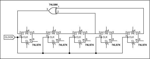
Figure 1. Simplified drawing of a LFSR.
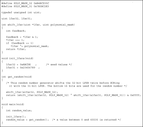
Figure 2. C code implementing a LFSR.
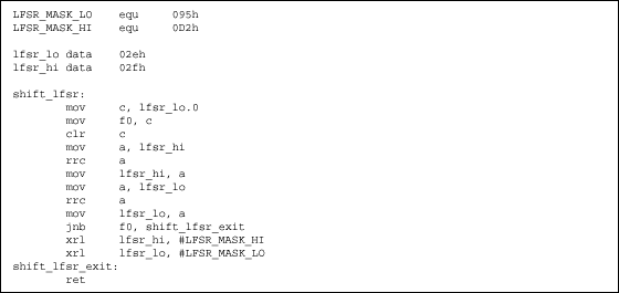
Figure 3. 8051 assembly code to implement a 16-bit LFSR with mask 0D295h.
Table 1. All 6th-degree primitive polynomials
Table 2. Polynomial information
Table 3. Sample masks and first four values output after initializing LFSR with one
Introduction
LFSRs (linear feedback shift registers) provide a simple means for generating nonsequential lists of numbers quickly on microcontrollers. Generating the pseudo-random numbers only requires a right-shift operation and an XOR operation. Figure 1 shows a 5-bit LFSR. Figure 2 shows an LFSR implementation in C, and Figure 3 shows a 16-bit LFSR implementation in 8051 assembly.LFSRs and polynomials
A LFSR is specified entirely by its polynomial. For example, a 6th-degree polynomial with every term present is represented with the equation x6 + x5 + x4 + x3 + x2 + x + 1. There are 2(6 - 1) = 32 different possible polynomials of this size. Just as with numbers, some polynomials are prime or primitive. We are interested in primitive polynomials because they will give us maximum length periods when shifting. A maximum length polynomial of degree n will have 2n - 1 different states. A new state is transitioned to after each shift. Consequently, a 6th-degree polynomial will have 31 different states. Every number between 1 and 31 will occur in the shift register before it repeats. In the case of primitive 6th-degree polynomials, there are only six. Table 1 lists all the primitive 6th-degree polynomials and their respective polynomial masks. The polynomial mask is created by taking the binary representation of the polynomial and truncating the right-most bit. The mask is used in the code that implements the polynomial. It takes n bits to implement the polynomial mask for an nth-degree polynomial.Every primitive polynomial will have an odd number of terms, which means that every mask for a primitive polynomial will have an even number of 1 bit. Every primitive polynomial also defines a second primitive polynomial, its dual. The dual can be found by subtracting the exponent from the degree of the polynomial for each term. For example, given the 6th-degree polynomial, x6 + x + 1, its dual is x6-6 + x6-1 + x6-0, which is equal to x6 + x5 + 1. In Table 1, polynomials 1 and 2, 3 and 4, 5 and 6 are the duals of each other.
Table 2 lists the period of each different size polynomial and the number of primitive polynomials that exist for each size. Table 3 lists one polynomial mask for each polynomial of a different size. It also shows the first four values that the LFSR will hold after consecutive shifts when the LFSR is initialized to one. This table should help to ensure that the implementation is correct.
The structure of a LFSR
LFSRs can never have the value of zero, since every shift of a zeroed LFSR will leave it as zero. The LFSR must be initialized, i.e., seeded, to a nonzero value. When the LFSR holds 1 and is shifted once, its value will always be the value of the polynomial mask. When the register is all zeros except the most significant bit, then the next several shifts will show the high bit shift to the low bit with zero fill. For example, any 8-bit shift register with a primitive polynomial will eventually generate the sequence 0x80, 0x40, 0x20, 0x10, 8, 4, 2, 1 and then the polynomial mask.Generating pseudo-random numbers with LFSR
In general, a basic LFSR does not produce very good random numbers. A better sequence of numbers can be improved by picking a larger LFSR and using the lower bits for the random number. For example, if you have a 10-bit LFSR and want an 8-bit number, you can take the bottom 8 bits of the register for your number. With this method you will see each 8-bit number four times and zero, three times, before the LFSR finishes one period and repeats. This solves the problem of getting zeros, but still the numbers do not exhibit very good statistical properties. Instead you can use a subset of the LFSR for a random number to increase the permutations of the numbers and improve the random properties of the LFSR output.Shifting the LFSR more than once before getting a random number also improves its statistical properties. Shifting the LFSR by a factor of its period will reduce the total period length by that factor. Table 2 has the factors of the periods.
The relatively short periods of the LFSRs can be solved by XORing the values of two or more different sized LFSRs together. The new period of these XORed LFSRs will be the LCM (least common multiple) of the periods. For example, the LCM of a primitive 4-bit and a primitive 6-bit LFSR is the LCM(15, 63), which is 315. When joining LFSRs in this way, be sure to use only the minimum number of bits of the LFSRs; it is a better practice to use less than that. With the 4- and 6-bit LFSRs, no more than the bottom 4 bits should be used. In Figure 2, the bottom 16 bits are used from 32- and 31-bit LFSRs. Note that XORing two LFSRs of the same size will not increase the period.
The unpredictability of the LFSRs can be increased by XORing a bit of "entropy" with the feedback term. Some care should be taken when doing this—there is a small chance that the LFSR will go to all zeros with the addition of the entropy bit. The zeroing of the LFSR will correct itself if entropy is added periodically. This method of XORing a bit with the feedback term is how CRCs (cyclic redundancy checks) are calculated.
Polynomials are not created equal. Some polynomials will definitely be better than others. Table 2 lists the number of primitive polynomials available for bit sizes up to 31 bits. Try different polynomials until you find one that meets your needs. The masks given in Table 3 were randomly selected.
All the basic statistical tests used for testing random number generators can be found in Donald Knuths, The Art of Computer Programming, Volume 2, Section 3.3. More extensive testing can be done using NIST's Statistical Test Suite. NIST also has several publications describing random number testing and references to other test software.

Figure 1. Simplified drawing of a LFSR.

Figure 2. C code implementing a LFSR.

Figure 3. 8051 assembly code to implement a 16-bit LFSR with mask 0D295h.
Table 1. All 6th-degree primitive polynomials
| Irreducible Polynomial | In Binary Form | Binary Mask | Mask | |
|
|
|
|
|
|
|
|
|
|
|
|
|
|
|
|
|
|
|
|
|
|
|
|
|
|
|
|
|
|
|
|
|
|
|
|
Table 2. Polynomial information
| Degree | Period | Factors of Period | No. of Primitive Polynomials of This Degree |
|
|
|
|
|
|
|
|
|
|
|
|
|
|
|
|
|
|
|
|
|
|
|
|
|
|
|
|
|
|
|
|
|
|
|
|
|
|
|
|
|
|
|
|
|
|
|
|
|
|
|
|
|
|
|
|
|
|
|
|
|
|
|
|
|
|
|
|
|
|
|
|
|
|
|
|
|
|
|
|
|
|
|
|
|
|
|
|
|
|
|
|
|
|
|
|
|
|
|
|
|
|
|
|
|
|
|
|
|
|
|
|
|
|
|
|
|
|
|
|
|
|
|
|
|
|
|
|
|
|
|
|
|
|
|
|
|
|
|
|
|
|
|
|
|
|
|
|
|
|
Table 3. Sample masks and first four values output after initializing LFSR with one
| Degree | Typical Mask | First Four Values in LFSR After Consecutive Shifts | |||
|
|
|
|
|
|
|
|
|
|
|
|
|
|
|
|
|
|
|
|
|
|
|
|
|
|
|
|
|
|
|
|
|
|
|
|
|
|
|
|
|
|
|
|
|
|
|
|
|
|
|
|
|
|
|
|
|
|
|
|
|
|
|
|
|
|
|
|
|
|
|
|
|
|
|
|
|
|
|
|
|
|
|
|
|
|
|
|
|
|
|
|
|
|
|
|
|
|
|
|
|
|
|
|
|
|
|
|
|
|
|
|
|
|
|
|
|
|
|
|
|
|
|
|
|
|
|
|
|
|
|
|
|
|
|
|
|
|
|
|
|
|
|
|
|
|
|
|
|
|
|
|
|
|
|
|
|
|
|
|
|
|
|
|
|
|
|
|
|
|
|
|
|
|
|
|
|
|
|
|
|
|
|
|
|
|
|
|
|
|
|
|
|
|
|
|
|
|
|
|
|
|
|
|
|
|
|
|
|
|
 电子发烧友App







评论